Steps in Machine Learning

Let us assume that we have a matrix of 1,000 training examples (houses) as rows, and 10 features (distance to downtown, sq. foot of house and no. of schools) as columns. The last column 'y' denotes the affordability of the house - expensive (denoted as 1) or affordable (denoted as 0). Following is a subset of the data -

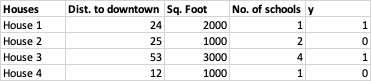
The above is our training set. Our aim is to predict the affordability of 50 houses for which we do not have the labels 'y'. That would be our test set.

Step 1: Initialization

We initialize an equation  y = σ(β0 + β1*x1 + β2*x2 ... β10*x10). β0 is the price of the house when we do not have any information on the features of the house, or the average cost of a house. x1, x2, x3... are the values of features listed in the table. The following variables are initialized to zero -

• β0, β1, β2 ... β10
• Cost function J
• dJ/dβ0, dJ/dβ1 ... dJ/dβ10 (which is the slope or derivative of cost function J with respect to dβX, where X = 0, 1, 2, 3 ... 10)

Step 2: Computation of Loss

We compute ŷ (pronounced as y-hat, which refers to the predicted y) using x1, x2, x3 ... and β0, β1, β2, β3 ... , where ŷ ranges between 0 and 1. This is done using the equation specified in Step 1.

Now that we know the values of ŷ and y, we compute the loss, and add it to the initialized cost function J. Loss is computed using the cross-entropy loss formula stated below -

loss = −(ylog(ŷ) + (1−y)log(1−ŷ)).

Step 3: Gradient Descent

We next compute the derivative of J with respect to z  (dJ/dz) where z = σ(β0 + β1*x1 + β2*x2 ...β10*x10, z being the affordability of a single house. Using dJ/dz, we further compute the derivative of J with respect to βX, and add them to initialized dJ/dβX (where X = 0, 1, 2 ... 10).

The above Steps 2 and 3 are implemented in a vectorized manner for all training examples.

Step 4: Update Parameters

The initialized βs get updated as follows :

β0 = β0 + (α * dJ/dβ0) / m

β1 = β1 + (α * dJ/dβ1) / m

'α' here can be set manually and helps determine the magnitude of coefficients (βs). Cost function J also gets updated as follows:

J = J/m

dJ/dβ0, dJ/dβ1, dJ/dβ2 ... are again set to 0. Values of J for each iteration are stored in a list, and J is reset to 0 as well.

Steps 2, 3 and 4 are repeated until the value of J is minimized (or until the total number of iterations are exhausted). In the end, we have the optimal values for β0, β1, β2 ... which may be used to make predictions on the test set.